Seasonality Of The Deposition Date

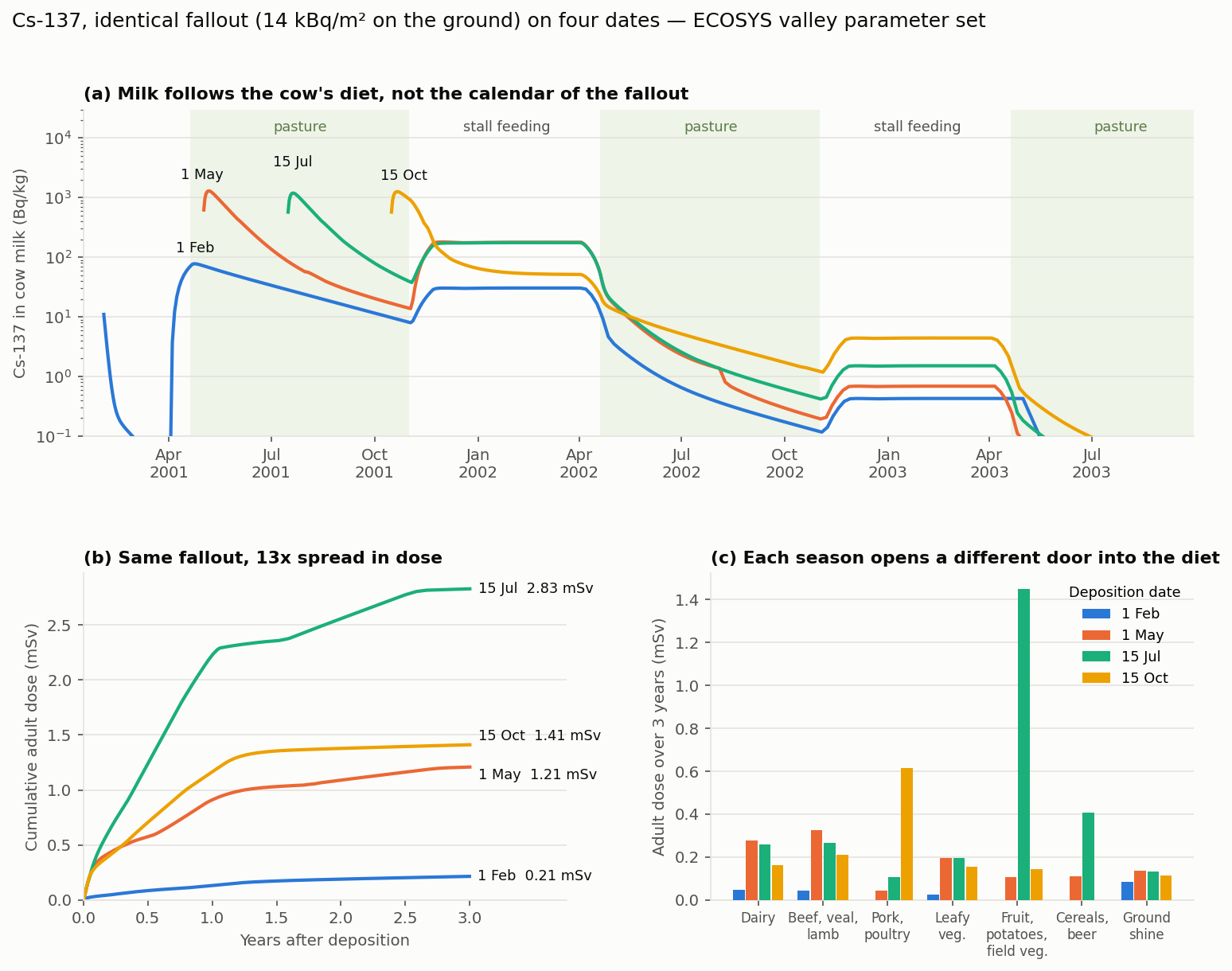
The same Cs-137 fallout gives very different doses depending on the calendar day it falls. This example deposits identical inputs on four dates in the default valley parameter set and follows each case for three years:

For complementary comparisons that hold the date fixed while varying nuclide, dry/wet route and rainfall, see Nuclides and Dry/Wet Deposition.

Date	Situation in the valley calendar
1 Feb	No plant growth; cows in the stall on stored hay, silage and grain
1 May	Young grass; cows have just moved to pasture (20 April)
15 Jul	Full canopy; cereals, potatoes and fruit are in or near harvest
15 Oct	Cereals and potatoes harvested; maize harvest starting; last weeks of grazing

Each event uses 100 Bq/m³ over one day, 10 kBq/m² wet deposition and 5 mm of rain. The ground receives 14.3 kBq/m² on every date. Only interception by vegetation changes with the season: 1 % for grass on 1 February and 22 % in mid-July.

from datetime import date

import astropy.units as u
import numpy as np

from ecosys import EcosysEngine
from ecosys.domain.events import DepositionEvent
from ecosys.domain.populations import PopulationCohorts
from ecosys.domain.request import SimulationRequest
from ecosys.domain.units import DOSE_UNIT

population = PopulationCohorts(
    initial_age=np.array([1.0, 30.0]) * u.year,
    population=np.array([1.0, 1.0]) * u.dimensionless_unscaled,
)
engine = EcosysEngine()
three_year_msv = {}
for day in (date(2001, 2, 1), date(2001, 5, 1), date(2001, 7, 15), date(2001, 10, 15)):
    event = DepositionEvent.from_constant_air_concentration(
        "cs_137", day, 100 * u.Bq / u.m**3, 1 * u.day, 10_000 * u.Bq / u.m**2, 5 * u.mm
    )
    request = SimulationRequest.on_default_grid(
        (event,), population, output_start_date=day, horizon_years=3
    )
    result = engine.run(request)
    three_year_msv[day] = result.per_capita.cumulative[-1].to_value(DOSE_UNIT) * 1000

adult = {day: dose[1] for day, dose in three_year_msv.items()}
assert max(adult, key=adult.get) == date(2001, 7, 15)
assert min(adult, key=adult.get) == date(2001, 2, 1)

The script seasonality/seasonality.py runs the same cases and draws the figure. It requires matplotlib, which ecosys does not install.

Results

Three-year cumulative effective dose, all supported pathways:

Deposition	Adult (mSv)	1-year-old (mSv)	Largest contributors (adult)
1 Feb	0.21	0.21	ground shine 40 %, milk 19 %, leafy vegetables 12 %
1 May	1.21	0.89	milk, meat and leafy vegetables
15 Jul	2.83	1.62	fruit, potatoes and field vegetables 51 %, cereals 14 %
15 Oct	1.41	0.70	pork 43 %

The same fallout gives a thirteen-fold range in adult dose. The date also determines which foods carry most of the dose.

Interpretation

Winter deposition is mostly lost. On 1 February the grass has almost no leaf area and intercepts 1 % of the deposit. Its concentration is high, because a small deposit sits on a small biomass, but no cow eats it: the ration is stored hay, maize silage and barley from the previous season. Milk shows only a short spike from cow inhalation of the cloud (panel a). The cows move to pasture from 1 April and are fully on grass by 20 April. By then 80 days of weathering (half-life 25 days) and growth dilution have removed about 97 % of the grass activity, and milk peaks at 78 Bq/kg instead of about 1300 Bq/kg. Leafy vegetables intercept normally in February, but winter consumption is scaled by 0.1 of the annual mean. Ground shine is similar on all dates, so it becomes the largest single pathway in this case.

Spring and summer deposition reaches milk within days. On 1 May and 15 July cows eat 75 kg/day of freshly contaminated grass, and milk exceeds 1000 Bq/kg within five days. It then falls with the weathering half-life. A second plateau follows each autumn (panel a) when the cows return to the stall. Their hay was dried from grass during the mid-May to mid-September preparation window, so the contamination is released with a delay of several months. The flat level reflects the fixed hay stock, which loses activity only by radioactive decay. The next year's pasture returns milk to a low, root-uptake-driven level.

Mid-July reaches the crops that people eat directly. On 15 July potatoes, fruiting vegetables and orchard fruit have a full canopy and are within their harvest windows. Leaf deposit translocates to the edible parts, and the harvested stock carries this activity through the year. This group alone accounts for 1.45 mSv. Panel (b) shows a second increase between about 1.6 and 2.5 years. That is wheat, harvested one to three weeks after the event and stored for 576 days as flour before consumption. Stored products can therefore give a significant dose long after fresh products are clean.

Mid-October affects the pig diet. Cereals and potatoes are harvested, but maize is not: its harvest runs from day 288 to 319, which starts on 15 October. Maize cobs reach about 1400 Bq/kg, and pigs eat 2.7 kg/day of them for a year. Pork is therefore 43 % of the October dose, compared with 4 % for the May deposit. Maize silage causes the first-winter milk plateau in panel (a). That winter's hay was made before the event and is uncontaminated.

Infants. The 1-year-old dose is about half the adult dose in July and October, when fruit, vegetables and pork dominate, and about 75 % in May, when milk carries more weight. This reflects the age-dependent consumption rates. In February ground shine dominates, and it depends little on age, so the two doses are nearly equal.

Model conventions

• The ground-shine source is the ground deposit plus the deposit on turf. It is therefore about 70 % larger for a spring or summer deposit than for a winter one (model reference, external ground dose).
• The diet is fixed: the model assumes locally produced food with no countermeasures. These results show the size of each pathway, which indicates where countermeasures would have most effect: keeping cows in the stall in May, delaying the July harvest, or controlling pig feed in October.
• The valley set has original-model reference runs for Cs-137. The mountain and Ticino/Valais sets have none, so the comparison below shows model behaviour only. See Validation Evidence.

Mountain Comparison

The mountain parameter set describes late vegetation at higher altitude. Its transfer factors and dose coefficients are the same as the valley's, and its human consumption and inhalation rates differ only marginally. The difference is the agricultural calendar: phenology (leaf area, biomass, growth rates), harvest windows, yields and the animal rations that follow the grazing season.

	Valley	Mountain
Grass growth starts	day 69 (10 Mar)	day 84 (25 Mar)
Cows move to pasture	1–20 Apr	25 Apr – 15 May
Cows return to stall	1–20 Nov	25 Oct – 5 Nov
Wheat and rye harvest	20 Jul – 5 Aug	5–20 Aug
Maize cob harvest	15 Oct – 15 Nov	15 Oct – 5 Nov
Yield: potatoes, orchard fruit (kg/m²)	3.8, 2.8	3.0, 2.0

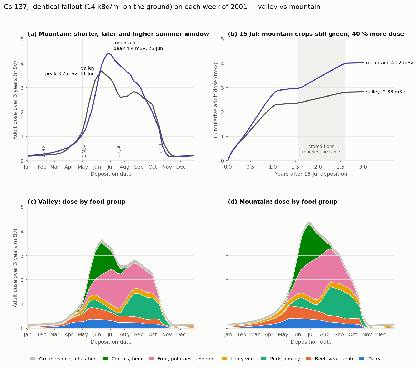
To compare the calendars rather than four sample dates, seasonality/mountain_comparison.py repeats the same deposit on every week of 2001 for both sets (about 90 s). The engine takes the parameter set as an argument:

from datetime import date

import astropy.units as u
import numpy as np

from ecosys import EcosysEngine
from ecosys.domain.events import DepositionEvent
from ecosys.domain.populations import PopulationCohorts
from ecosys.domain.request import SimulationRequest
from ecosys.domain.units import DOSE_UNIT

adult = PopulationCohorts(np.array([30.0]) * u.year, np.array([1.0]) * u.dimensionless_unscaled)
day = date(2001, 7, 15)
event = DepositionEvent.from_constant_air_concentration(
    "cs_137", day, 100 * u.Bq / u.m**3, 1 * u.day, 10_000 * u.Bq / u.m**2, 5 * u.mm
)
request = SimulationRequest.on_default_grid((event,), adult, output_start_date=day, horizon_years=3)
msv = {
    name: EcosysEngine(parameter_set=name).run(request).per_capita.cumulative[-1, 0].to_value(DOSE_UNIT) * 1000
    for name in ("valley", "mountain")
}
assert msv["mountain"] > 1.3 * msv["valley"]

Three-year cumulative dose for the four example dates:

Deposition	Valley adult (mSv)	Mountain adult (mSv)	Valley 1-year-old (mSv)	Mountain 1-year-old (mSv)
1 Feb	0.21	0.26	0.20	0.23
1 May	1.21	1.08	0.89	0.83
15 Jul	2.83	4.02	1.62	2.23
15 Oct	1.41	1.30	0.70	0.68

In the weekly sweep the adult dose exceeds 2 mSv from 14 May to 1 October in the valley (21 weeks) and from 21 May to 24 September in the mountains (19 weeks). The valley peak is 3.7 mSv for a deposit on 11 June; the mountain peak is 4.4 mSv on 25 June. Averaged over all deposition dates, the mountain dose is only 10 % higher (1.57 vs 1.43 mSv). The mountain calendar makes the sensitive window shorter, later and higher. It does not make every date worse.

Interpretation

The summer peak is set by the cereal harvest. Cereals are the largest group at both peaks (green in panels c and d). For wheat and rye the fraction of leaf deposit that reaches the grain is largest, 0.10, when harvest follows the deposit by 30–50 days, and it falls to about 0.02 at 90 days. The valley cereal harvest starts on 20 July, so a deposit in early to mid-June is the worst case. In the mountains harvest starts on 5 August, and the worst case moves two weeks later. The flour is stored for 576 days, so this dose arrives in the second and third year (panel b).

Mid-July hits green mountain crops and ripening valley crops. The largest difference is for a 15 July deposit: 4.02 vs 2.83 mSv. The valley cereals are ripening and their leaf area has dropped, so they intercept only 5–8 % of the deposit. Mountain cereals are still green and intercept 9–13 %, with more time left before harvest. Cereals therefore contribute 0.95 mSv in the mountains against 0.36 mSv in the valley. Fruit, potatoes and field vegetables intercept the same fraction in both sets, but the mountain yields are lower (for example 2.0 vs 2.8 kg/m² for orchard fruit). The same deposit is therefore spread over less produce, which raises the concentration. Panel (b) shows the two contributions: a steeper first year from fresh produce and a larger step when the stored flour is eaten.

The mountain dose drops out earlier in autumn. Mountain cows return to the stall from 25 October, and the maize cob harvest ends on 5 November instead of 15 November. A deposit on 5 November gives 0.16 mSv in the mountains and 0.33 mSv in the valley. Most of the valley difference is pork, because the last valley maize is still in the field.

Late winter is slightly worse in the mountains. A deposit between February and March gives up to 40 % more dose in the mountains, although the absolute values stay below 0.5 mSv. Mountain grass starts growing two weeks later, so a similar deposit sits on much less biomass. For a 26 February deposit the grass reaches 4100 Bq/kg on 10 April, against 760 Bq/kg in the valley. The cows move to pasture later, but by then the grass still has 900 instead of 530 Bq/kg, and milk peaks at 180 instead of 110 Bq/kg. Leafy vegetables add to this: the mountain harvest starts on 25 May instead of 1 May, so the crop that received the deposit in winter is still eaten after summer consumption rates begin on 2 May.

1 May is slightly lower in the mountains. On 1 May mountain cows are partly on pasture, and milk peaks at 870 instead of 1290 Bq/kg. Potatoes, fruit and most cereals have barely emerged, so few crops receive the deposit. Over three years, milk and meat end up slightly higher. Mountain grass has less biomass in May, so the hay made from it is more contaminated (7600 vs 7100 Bq/kg), and the stall season that uses it starts a week earlier. The higher winter milk offsets the lower spring peak. The crop pathways are smaller, however, and the total is 1.08 against 1.21 mSv.